Sections in this Chapter:
Upon the feedbacks and requests from readers of the first few chapters, I made a decision to spend a whole chapter in the introduction of data.table and pandas. Of course, there are many other great data analysis tools in both R and Python. For example, many R users like using dplyr to build up data analysis pipelines. The performance of data.table is superior and that is the main reason I feel there is no need to use other tools for the same tasks in R. But if you are a big fan for the pipe operator \%>\% you may use data.table and dplyr together. Regarding the big data ecosystem, Apache Spark has API in both R and Python. Recently, there are also some emerging projects aiming at better usability and performance, such as Apache Arrow1, Modin2.
SQL
Similar to the previous chapters, I will introduce the tools side by side. However, I feel before diving into the world of data.table and pandas, it is better to talk a little bit about SQL3. SQL is a Query language designed for managing data in relational database management system (RDBMS). Some of the most popular RDBMSs include MS SQL Server, MySQL, PostgreSQL, etc. Different RDBMSs may use SQL languages with major or subtle differences.
If you have never used RDBMS you may wonder why we need it?
- first, we need a system to store the data;
- second, we also need a system that allows us to easily access, manage and update the data.
Let’s assume there is a table mtcars in a database (I’m using sqlite3 in this book) and see some simple tasks we can do with SQL queries.
| name | mpg | cyl | disp | hp | drat | wt | qsec | vs | am | gear | carb |
| Mazda RX4 | 21 | 6 | 160 | 110 | 3.9 | 2.62 | 16.46 | 0 | 1 | 4 | 4 |
| Mazda RX4 Wag | 21 | 6 | 160 | 110 | 3.9 | 2.875 | 17.02 | 0 | 1 | 4 | 4 |
| Datsun 710 | 22.8 | 4 | 108 | 93 | 3.85 | 2.32 | 18.61 | 1 | 1 | 4 | 1 |
| Hornet 4 Drive | 21.4 | 6 | 258 | 110 | 3.08 | 3.215 | 19.44 | 1 | 0 | 3 | 1 |
| Hornet Sportabout | 18.7 | 8 | 360 | 175 | 3.15 | 3.44 | 17.02 | 0 | 0 | 3 | 2 |
| Valiant | 18.1 | 6 | 225 | 105 | 2.76 | 3.46 | 20.22 | 1 | 0 | 3 | 1 |
| Duster 360 | 14.3 | 8 | 360 | 245 | 3.21 | 3.57 | 15.84 | 0 | 0 | 3 | 4 |
| Merc 240D | 24.4 | 4 | 146.7 | 62 | 3.69 | 3.19 | 20 | 1 | 0 | 4 | 2 |
| Merc 230 | 22.8 | 4 | 140.8 | 95 | 3.92 | 3.15 | 22.9 | 1 | 0 | 4 | 2 |
| Merc 280 | 19.2 | 6 | 167.6 | 123 | 3.92 | 3.44 | 18.3 | 1 | 0 | 4 | 4 |
| Merc 280C | 17.8 | 6 | 167.6 | 123 | 3.92 | 3.44 | 18.9 | 1 | 0 | 4 | 4 |
| Merc 450SE | 16.4 | 8 | 275.8 | 180 | 3.07 | 4.07 | 17.4 | 0 | 0 | 3 | 3 |
| Merc 450SL | 17.3 | 8 | 275.8 | 180 | 3.07 | 3.73 | 17.6 | 0 | 0 | 3 | 3 |
| Merc 450SLC | 15.2 | 8 | 275.8 | 180 | 3.07 | 3.78 | 18 | 0 | 0 | 3 | 3 |
| Cadillac Fleetwood | 10.4 | 8 | 472 | 205 | 2.93 | 5.25 | 17.98 | 0 | 0 | 3 | 4 |
| Lincoln Continental | 10.4 | 8 | 460 | 215 | 3 | 5.424 | 17.82 | 0 | 0 | 3 | 4 |
| Chrysler Imperial | 14.7 | 8 | 440 | 230 | 3.23 | 5.345 | 17.42 | 0 | 0 | 3 | 4 |
| Fiat 128 | 32.4 | 4 | 78.7 | 66 | 4.08 | 2.2 | 19.47 | 1 | 1 | 4 | 1 |
| Honda Civic | 30.4 | 4 | 75.7 | 52 | 4.93 | 1.615 | 18.52 | 1 | 1 | 4 | 2 |
| Toyota Corolla | 33.9 | 4 | 71.1 | 65 | 4.22 | 1.835 | 19.9 | 1 | 1 | 4 | 1 |
| Toyota Corona | 21.5 | 4 | 120.1 | 97 | 3.7 | 2.465 | 20.01 | 1 | 0 | 3 | 1 |
| Dodge Challenger | 15.5 | 8 | 318 | 150 | 2.76 | 3.52 | 16.87 | 0 | 0 | 3 | 2 |
| AMC Javelin | 15.2 | 8 | 304 | 150 | 3.15 | 3.435 | 17.3 | 0 | 0 | 3 | 2 |
| Camaro Z28 | 13.3 | 8 | 350 | 245 | 3.73 | 3.84 | 15.41 | 0 | 0 | 3 | 4 |
| Pontiac Firebird | 19.2 | 8 | 400 | 175 | 3.08 | 3.845 | 17.05 | 0 | 0 | 3 | 2 |
| Fiat X1-9 | 27.3 | 4 | 79 | 66 | 4.08 | 1.935 | 18.9 | 1 | 1 | 4 | 1 |
| Porsche 914-2 | 26 | 4 | 120.3 | 91 | 4.43 | 2.14 | 16.7 | 0 | 1 | 5 | 2 |
| Lotus Europa | 30.4 | 4 | 95.1 | 113 | 3.77 | 1.513 | 16.9 | 1 | 1 | 5 | 2 |
| Ford Pantera L | 15.8 | 8 | 351 | 264 | 4.22 | 3.17 | 14.5 | 0 | 1 | 5 | 4 |
| Ferrari Dino | 19.7 | 6 | 145 | 175 | 3.62 | 2.77 | 15.5 | 0 | 1 | 5 | 6 |
| Maserati Bora | 15 | 8 | 301 | 335 | 3.54 | 3.57 | 14.6 | 0 | 1 | 5 | 8 |
| Volvo 142E | 21.4 | 4 | 121 | 109 | 4.11 | 2.78 | 18.6 | 1 | 1 | 4 | 2 |
1 sqlite> select * from mtcars limit 2;
2 name,mpg,cyl,disp,hp,drat,wt,qsec,vs,am,gear,carb
3 "Mazda RX4",21,6,160,110,3.9,2.62,16.46,0,1,4,4
4 "Mazda RX4 Wag",21,6,160,110,3.9,2.875,17.02,0,1,4,4
In the example above, I select two rows from the table using the syntax select from. The keyword limit in sqlite specifies the number of rows to return. In other RMDBSs, we may need to use top instead.
It is straightforward to select on conditions with the where keyword.
1 sqlite> select mpg,cyl from mtcars where name = 'Mazda RX4 Wag';
2 mpg,cyl
3 21,6
We can definitely use more conditions with the where clause.
 1 sqlite> .mode column -- make the output aligned; and yes we use '--' to start comment in many SQL languages
 2 sqlite> select name, mpg, cyl,vs,am from mtcars where vs=1 and am=1;
 3 name        mpg         cyl         vs          am
 4 ----------  ----------  ----------  ----------  ----------
 5 Datsun 710  22.8        4           1           1
 6 Fiat 128    32.4        4           1           1
 7 Honda Civi  30.4        4           1           1
 8 Toyota Cor  33.9        4           1           1
 9 Fiat X1-9   27.3        4           1           1
10 Lotus Euro  30.4        4           1           1
11 Volvo 142E  21.4        4           1           1
Staring at the example above, what are we doing? Actually, we are just accessing specific rows and columns from the table in database with select from where.
We can also do something a bit of more fancy, for example, to get the maximum, the minimum and the average of mpg for all vehicles grouped by the number of cylinders.
1 sqlite> select cyl, max(mpg) as max, min(mpg) as min, avg(mpg) as avg from mtcars group by cyl order by cyl;
2 cyl         max         min         avg
3 ----------  ----------  ----------  ----------------
4 4           33.9        21.4        26.6636363636364
5 6           21.4        17.8        19.7428571428571
6 8           19.2        10.4        15.1
In the above example, there are a few things worth noting. We use as to create an alias for a variable; we group the original rows by the number of cylinders with the keyword group by; and we sort the output rows with the keyword order by. max, min and avg are all built-in functions that we can use directly.
It is also possible to have user-defined functions in SQL as what we usually do in other programming languages.
SQL is a very powerful tool for data analysis, but it works on RMDBS and generally we can’t apply R or Python functions to the database tables directly. Many practitioners in data science have to work with database at times but more often they need to work in a programming languages such as R or Python. We have introduced the data.frame in both R and Python in previous chapters. A data.frame is just like a database table that you may operate within the corresponding language. Usually a data.frame is stored in memory, but of course it can also be deserialized for storage in hard disks.
With the data.frame-like objects, we could build up a better data processing pipeline by only reading the original data from the database and storing the final output to the database if necessary. Most of works we can do with data.frame-like objects may also be done in RMBDS with SQL. But they may require intense interactions with a database, which is not preferred if they could be avoided.
Now, let’s get started with data.table and pandas. In this book, I will use data.table 1.12.0 and pandas 0.24.0.
Get started with data.table & pandas
1 > library(data.table)
2 data.table 1.12.0 Latest news: r-datatable.com1 >>> import pandas as pd
2 >>> pd.__version__
3 '0.24.2'I have saved the mtcars data to a csv4 file (code/chapter3/mtcars.csv), which is loaded from R 3.5.1. Although the mtcars data is loaded into R environment by default, let’s load the data by reading the raw csv file for learning purpose.
1 > mtcars_dt=fread('mtcars.csv')
2 > head(mtcars_dt)
3                 name  mpg cyl disp  hp drat    wt  qsec vs am gear carb
4 1:         Mazda RX4 21.0   6  160 110 3.90 2.620 16.46  0  1    4    4
5 2:     Mazda RX4 Wag 21.0   6  160 110 3.90 2.875 17.02  0  1    4    4
6 3:        Datsun 710 22.8   4  108  93 3.85 2.320 18.61  1  1    4    1
7 4:    Hornet 4 Drive 21.4   6  258 110 3.08 3.215 19.44  1  0    3    1
8 5: Hornet Sportabout 18.7   8  360 175 3.15 3.440 17.02  0  0    3    2
9 6: Valiant 18.1 6 225 105 2.76 3.460 20.22 1 0 3 1 1 >>> import pandas as pd
2 >>> mtcars_df=pd.read_csv('mtcars.csv')
3 >>> mtcars_df.head(5)
4 name mpg cyl disp hp ... qsec vs am gear carb
5 0 Mazda RX4 21.0 6 160.0 110 ... 16.46 0 1 4 4
6 1 Mazda RX4 Wag 21.0 6 160.0 110 ... 17.02 0 1 4 4
7 2 Datsun 710 22.8 4 108.0 93 ... 18.61 1 1 4 1
8 3 Hornet 4 Drive 21.4 6 258.0 110 ... 19.44 1 0 3 1
9 4 Hornet Sportabout 18.7 8 360.0 175 ... 17.02 0 0 3 2
10
11 [5 rows x 12 columns]The type of mtcars_dt is data.table, not data.frame. Here we use the fread function from data.table to read a file and the output type is a data.table directly. Regarding reading csv in R, a very good package is readr for very large files, but the output has a data.frame type. In practice, it is very common to convert a data.frame to data.table with the function as.data.table.
Indexing & selecting data
Before to introduce the indexing rules in data.table and pandas, it’s better to understand the key in data.table and the index in pandas.
What is the key in a data.table? We have talked about RMDBS and SQL in the previous section. With select from where we can easily access specific rows satisfying certain conditions. When the database table is too large, a database index is used to improve the performance of data retrieval operations. Essentially, a database index is a data structure, and to maintain the data structure additional cost (for example, space) may be required. The reason to use key in data.table and index in pandas is very similar. Now let’s see how to set key and index.
 1 > setkey(mtcars_dt, name)
 2 > key(mtcars_dt)
 3 [1] "name"
 4 > head(mtcars_dt, 5)
 5                  name  mpg cyl disp  hp drat    wt  qsec vs am gear carb
 6 1:        AMC Javelin 15.2   8  304 150 3.15 3.435 17.30  0  0    3    2
 7 2: Cadillac Fleetwood 10.4   8  472 205 2.93 5.250 17.98  0  0    3    4
 8 3:         Camaro Z28 13.3   8  350 245 3.73 3.840 15.41  0  0    3    4
 9 4:  Chrysler Imperial 14.7   8  440 230 3.23 5.345 17.42  0  0    3    4
10 5: Datsun 710 22.8 4 108 93 3.85 2.320 18.61 1 1 4 1 1 >>> mtcars_df.set_index('name', inplace=True)
2 >>> mtcars_df.index.name
3 'name'
4 >>> mtcars_df.head(5)
5 mpg cyl disp hp drat ... qsec vs am gear carb
6 name ...
7 Mazda RX4 21.0 6 160.0 110 3.90 ... 16.46 0 1 4 4
8 Mazda RX4 Wag 21.0 6 160.0 110 3.90 ... 17.02 0 1 4 4
9 Datsun 710 22.8 4 108.0 93 3.85 ... 18.61 1 1 4 1
10 Hornet 4 Drive 21.4 6 258.0 110 3.08 ... 19.44 1 0 3 1
11 Hornet Sportabout 18.7 8 360.0 175 3.15 ... 17.02 0 0 3 2There are quite a few things worth noting from the above code snippets. When we use the setkey function the quotes for the column name is optional. So setkey(mtcars_dt, name) is equivalent to setkey(mtcars_dt, 'name'). But in pandas, quotes are required. The effect of setkey is in place, which means no copies of the data made at all. But in pandas, by default set_index set the index on a copy of the data and the modified copy is returned. Thus, in order to make the effect in place, we have the set the argument inplace=True explicitly. Another difference is that setkey would sort the original data in place automatically but set_index does not. It’s also worth noting every pandas data.frame has an index; and by default it is numpy.arange(n) where n is the number of rows. But there is no default key in a data.table.
In the above example, we only use a single column as the key/index. It is possible to use multiple columns as well.
1 > setkeyv(mtcars_dt, c('cyl','gear'))
2 > key(mtcars_dt)
3 [1] "cyl" "gear"1 >>> mtcars_df.set_index([ 'cyl', 'gear'], inplace=True)
2 >>> mtcars_df.index.names
3 FrozenList(['cyl', 'gear'])To use multiple columns as the key in data.table, we use the function setkeyv. It is also interesting that we have to use index.names rather than index.name to get the multiple column names of the index (which is called MultiIndex) in pandas. There are duplicated combinations of (cyl, gear) in the data, which implies key or index could be duplicated.
Once the key/index set, we can access rows with given the indices fast.
 1 > mtcars_dt['Merc 230']
 2        name  mpg cyl  disp hp drat   wt qsec vs am gear carb
 3 1: Merc 230 22.8   4 140.8 95 3.92 3.15 22.9  1  0    4    2
 4 > mtcars_dt[c('Merc 230','Camaro Z28')] # multiple values of a single index
 5          name  mpg cyl  disp  hp drat   wt  qsec vs am gear carb
 6 1:   Merc 230 22.8   4 140.8  95 3.92 3.15 22.90  1  0    4    2
 7 2: Camaro Z28 13.3   8 350.0 245 3.73 3.84 15.41  0  0    3    4
 8 > setkeyv(mtcars_dt,c('cyl','gear'))
 9 > mtcars_dt[.(6,4)] # work with key vector using .()
10             name  mpg cyl  disp  hp drat    wt  qsec vs am gear carb
11 1:     Mazda RX4 21.0   6 160.0 110 3.90 2.620 16.46  0  1    4    4
12 2: Mazda RX4 Wag 21.0   6 160.0 110 3.90 2.875 17.02  0  1    4    4
13 3:      Merc 280 19.2   6 167.6 123 3.92 3.440 18.30  1  0    4    4
14 4:     Merc 280C 17.8   6 167.6 123 3.92 3.440 18.90  1  0    4    4
15 > mtcars_dt[.(c(6,8),c(4,3))] # key vector with multiple values
16                    name  mpg cyl  disp  hp drat    wt  qsec vs am gear carb
17  1:           Mazda RX4 21.0   6 160.0 110 3.90 2.620 16.46  0  1    4    4
18  2:       Mazda RX4 Wag 21.0   6 160.0 110 3.90 2.875 17.02  0  1    4    4
19  3:            Merc 280 19.2   6 167.6 123 3.92 3.440 18.30  1  0    4    4
20  4:           Merc 280C 17.8   6 167.6 123 3.92 3.440 18.90  1  0    4    4
21  5:         AMC Javelin 15.2   8 304.0 150 3.15 3.435 17.30  0  0    3    2
22  6:  Cadillac Fleetwood 10.4   8 472.0 205 2.93 5.250 17.98  0  0    3    4
23  7:          Camaro Z28 13.3   8 350.0 245 3.73 3.840 15.41  0  0    3    4
24  8:   Chrysler Imperial 14.7   8 440.0 230 3.23 5.345 17.42  0  0    3    4
25  9:    Dodge Challenger 15.5   8 318.0 150 2.76 3.520 16.87  0  0    3    2
26 10:          Duster 360 14.3   8 360.0 245 3.21 3.570 15.84  0  0    3    4
27 11:   Hornet Sportabout 18.7   8 360.0 175 3.15 3.440 17.02  0  0    3    2
28 12: Lincoln Continental 10.4   8 460.0 215 3.00 5.424 17.82  0  0    3    4
29 13:          Merc 450SE 16.4   8 275.8 180 3.07 4.070 17.40  0  0    3    3
30 14:          Merc 450SL 17.3   8 275.8 180 3.07 3.730 17.60  0  0    3    3
31 15:         Merc 450SLC 15.2   8 275.8 180 3.07 3.780 18.00  0  0    3    3
32 16:    Pontiac Firebird 19.2   8 400.0 175 3.08 3.845 17.05  0  0    3    2
Here is a bit of explanation for the code above. We can simply use [] to access the rows with the specified key values if the key has a character type. But if the key has a numeric type, list() is required to enclose the key values. In data.table, .() is just an alias of list(), which means we would get the same results with mtcars_dt[list(6,4)]. Of course, we can use also do mtcars_dt[.('Merc 230')] which is equivalent to mtcars_dt[.('Merc 230')].
 1 >>> mtcars_df.loc['Merc 230']
 2 mpg      22.80
 3 cyl       4.00
 4 disp    140.80
 5 hp       95.00
 6 drat      3.92
 7 wt        3.15
 8 qsec     22.90
 9 vs        1.00
10 am        0.00
11 gear      4.00
12 carb      2.00
13 Name: Merc 230, dtype: float64
14 >>> mtcars_df.loc[['Merc 230','Camaro Z28']] # multiple values of a single index
15              mpg  cyl   disp   hp  drat    wt   qsec  vs  am  gear  carb
16 name
17 Merc 230    22.8    4  140.8   95  3.92  3.15  22.90   1   0     4     2
18 Camaro Z28  13.3    8  350.0  245  3.73  3.84  15.41   0   0     3     4
19
20 mtcars_df.set_index(['cyl','gear'],inplace=True)
21 >>> mtcars_df.loc[(6,4)] # work with MultiIndex using ()
22            mpg   disp   hp  drat     wt   qsec  vs  am  carb
23 cyl gear
24 6   4     21.0  160.0  110  3.90  2.620  16.46   0   1     4
25     4     21.0  160.0  110  3.90  2.875  17.02   0   1     4
26     4     19.2  167.6  123  3.92  3.440  18.30   1   0     4
27     4     17.8  167.6  123  3.92  3.440  18.90   1   0     4
28 >>> # you may notice that the name column disappeared; that would be explained later
29 >>> mtcars_df.loc[[(6,4),(8,3)]] # MultiIndex with multiple values
30            mpg   disp   hp  drat     wt   qsec  vs  am  carb
31 cyl gear
32 6   4     21.0  160.0  110  3.90  2.620  16.46   0   1     4
33     4     21.0  160.0  110  3.90  2.875  17.02   0   1     4
34     4     19.2  167.6  123  3.92  3.440  18.30   1   0     4
35     4     17.8  167.6  123  3.92  3.440  18.90   1   0     4
36 8   3     18.7  360.0  175  3.15  3.440  17.02   0   0     2
37     3     14.3  360.0  245  3.21  3.570  15.84   0   0     4
38     3     16.4  275.8  180  3.07  4.070  17.40   0   0     3
39     3     17.3  275.8  180  3.07  3.730  17.60   0   0     3
40     3     15.2  275.8  180  3.07  3.780  18.00   0   0     3
41     3     10.4  472.0  205  2.93  5.250  17.98   0   0     4
42     3     10.4  460.0  215  3.00  5.424  17.82   0   0     4
43     3     14.7  440.0  230  3.23  5.345  17.42   0   0     4
44     3     15.5  318.0  150  2.76  3.520  16.87   0   0     2
45     3     15.2  304.0  150  3.15  3.435  17.30   0   0     2
46     3     13.3  350.0  245  3.73  3.840  15.41   0   0     4
47     3     19.2  400.0  175  3.08  3.845  17.05   0   0     2
Compared to data.table, we need to use the loc method when accessing rows based on index. The loc method also takes boolean conditions.
1 >>> mtcars_df.loc[mtcars_df.mpg>30] # select the vehicles with mpg>30
2            mpg  disp   hp  drat     wt   qsec  vs  am  carb
3 cyl gear
4 4   4     32.4  78.7   66  4.08  2.200  19.47   1   1     1
5     4     30.4  75.7   52  4.93  1.615  18.52   1   1     2
6     4     33.9  71.1   65  4.22  1.835  19.90   1   1     1
7     5     30.4  95.1  113  3.77  1.513  16.90   1   1     2
When using boolean conditions, loc could be ignored for convenience.
1 >>> mtcars_df[mtcars_df.mpg>30] # ignore loc with boolean conditions
2            mpg  disp   hp  drat     wt   qsec  vs  am  carb
3 cyl gear
4 4   4     32.4  78.7   66  4.08  2.200  19.47   1   1     1
5     4     30.4  75.7   52  4.93  1.615  18.52   1   1     2
6     4     33.9  71.1   65  4.22  1.835  19.90   1   1     1
7     5     30.4  95.1  113  3.77  1.513  16.90   1   1     2
If the key/index is not needed, we can remove the key or reset the index. For data.table we can set a new key to override the existing one which then becomes a column. But in pandas, set_index method removes the exiting index which also disappears from the data.frame.
 1 > key(mtcars_dt)
 2 [1] "cyl"  "gear"
 3 > setkey(mtcars_dt, NULL) # remove the existing key
 4 > key(mtcars_dt)
 5 NULL
 6 > setkey(mtcars_dt, 'gear')
 7 > key(mtcars_dt)
 8 [1] "gear"
 9 > setkey(mtcars_dt, 'name') # override the existing key
10 > key(mtcars_dt)
11 [1] "name" 1 >>> mtcars_df.index.names
2 FrozenList(['cyl', 'gear'])
3 >>> mtcars_df.reset_index(inplace=True) # remove the existing index
4 >>> mtcars_df.index.names
5 FrozenList([None])
6 >>> mtcars_df.set_index(['gear'], inplace=True)
7 >>> mtcars_df.index.name
8 'gear'
9 >>> mtcars_df.columns # list all columns
10 Index(['cyl', 'name', 'mpg', 'disp', 'hp', 'drat', 'wt', 'qsec', 'vs', 'am',
11 'carb'],
12 dtype='object')
13 >>> mtcars_df.set_index('name', inplace=True)
14 >>> mtcars_df.columns # the name column disappears
15 Index(['cyl', 'mpg', 'disp', 'hp', 'drat', 'wt', 'qsec', 'vs', 'am', 'carb'], dtype='object')In Chapter 1, we introduced integer-based indexing for list/vector. It is also applicable to data frame and data.table
1 > mtcars_dt=fread('mtcars.csv')
2 > mtcars_dt[c(1,2,6),]
3             name  mpg cyl disp  hp drat    wt  qsec vs am gear carb
4 1:     Mazda RX4 21.0   6  160 110 3.90 2.620 16.46  0  1    4    4
5 2: Mazda RX4 Wag 21.0   6  160 110 3.90 2.875 17.02  0  1    4    4
6 3: Valiant 18.1 6 225 105 2.76 3.460 20.22 1 0 3 11 >>> mtcars_df=pd.read_csv('mtcars.csv')
2 >>> mtcars_df.iloc[[0,1,5]] # again, indices in python are zero-based.
3 name mpg cyl disp hp ... qsec vs am gear carb
4 0 Mazda RX4 21.0 6 160.0 110 ... 16.46 0 1 4 4
5 1 Mazda RX4 Wag 21.0 6 160.0 110 ... 17.02 0 1 4 4
6 5 Valiant 18.1 6 225.0 105 ... 20.22 1 0 3 1So far we have seen how to access specific rows. What about columns? Accessing columns in data.table and pandas is quite straightforward. For data.table, we can use \$ sign to access a single column or a vector to specify multiple columns inside []. For data.frame in pandas, we can use . to access a single column or a list to specify multiple columns inside [].
1 > head(mtcars_dt$mpg,5) # access a single column
2 [1] 21.0 21.0 22.8 21.4 18.7}
3 > mtcars_dt[1:5,c('mpg', 'gear')]
4     mpg gear
5 1: 21.0    4
6 2: 21.0    4
7 3: 22.8    4
8 4: 21.4    3
9 5: 18.7 3 1 >>> mtcars_df.iloc[0:5 ].mpg.values
2 array([21. , 21. , 22.8, 21.4, 18.7])
3 Name: mpg, dtype: float64
4 >>> mtcars_df[['mpg', 'gear']].head(5)
5 mpg gear
6 0 21.0 4
7 1 21.0 4
8 2 22.8 4
9 3 21.4 3
10 4 18.7 3In addition to passing a vector to access multiple columns in data.table, we can also use the .(variable_1,variable_2,...).
1 > mtcars_dt[1:5,.(mpg,cyl,hp)] # without quotes for variables
2     mpg cyl hp
3 1: 21.5   4 97
4 2: 22.8   4 93
5 3: 24.4   4 62
6 4: 22.8   4 95
7 5: 32.4   4 66
It is also possible to do integer-based columns slicing.
1 > mtcars_dt[1:5,c(2,5,6)] # the 2nd, the 5th and the 6th column
2     mpg  hp drat
3 1: 21.0 110 3.90
4 2: 21.0 110 3.90
5 3: 22.8  93 3.85
6 4: 21.4 110 3.08
7 5: 18.7 175 3.151 >>> mtcars_df.iloc[0:5,[1,4,5]] # the 2nd, the 5th and the 6th column
2 mpg hp drat
3 0 21.0 110 3.90
4 1 21.0 110 3.90
5 2 22.8 93 3.85
6 3 21.4 110 3.08
7 4 18.7 175 3.15To access specific rows and specific columns, there are two strategies:
- select rows and then select columns in a chain;
- select rows and columns simultaneously.
Let’s see some examples.
 1 > mtcars_dt=fread('mtcars.csv')
 2 > setkey(mtcars_dt,'gear')
 3 > mtcars_dt[.(6),c('mpg','cyl','hp')] # use strategy 2;
 4     mpg cyl  hp
 5 1: 21.4   6 110
 6 2: 18.1   6 105
 7 3: 21.0   6 110
 8 4: 21.0   6 110
 9 5: 19.2   6 123
10 6: 17.8   6 123
11 7: 19.7   6 175
12 > mtcars_dt[.(6)][,c('mpg','cyl','hp')] # use strategy 1;
13     mpg cyl  hp
14 1: 21.4   6 110
15 2: 18.1   6 105
16 3: 21.0   6 110
17 4: 21.0   6 110
18 5: 19.2   6 123
19 6: 17.8   6 123
20 7: 19.7 6 175 1 >>> mtcars_df=pd.read_csv('mtcars.csv')
2 >>> mtcars_df.set_index('cyl', inplace=True)
3 >>> mtcars_df.loc[6,['mpg','hp']] # use strategy 2; we can't list the index as a normal column; while a key in data.table is still a normal column
4 mpg hp
5 cyl
6 6 21.0 110
7 6 21.0 110
8 6 21.4 110
9 6 18.1 105
10 6 19.2 123
11 6 17.8 123
12 6 19.7 175
13 >>> mtcars_df.loc[6][['mpg','hp']] # us strategy 1
14 mpg hp
15 cyl
16 6 21.0 110
17 6 21.0 110
18 6 21.4 110
19 6 18.1 105
20 6 19.2 123
21 6 17.8 123
22 6 19.7 175As we have seen, using the setkey function for data.table sorts the data.table automatically. However, sorting is not always desired. In data.table, there is another function setindex/setindexv which has similar effects to setkey/setkeyv but doesn’t sort the data.table. In addition, one data.table could have multiple indices, but it cannot have multiple keys.
 1 > setindex(mtcars_dt,'cyl')
 2 > head(mtcars_dt,5) # not sorted by the index
 3                 name  mpg cyl disp  hp drat    wt  qsec vs am gear carb
 4 1:         Mazda RX4 21.0   6  160 110 3.90 2.620 16.46  0  1    4    4
 5 2:     Mazda RX4 Wag 21.0   6  160 110 3.90 2.875 17.02  0  1    4    4
 6 3:        Datsun 710 22.8   4  108  93 3.85 2.320 18.61  1  1    4    1
 7 4:    Hornet 4 Drive 21.4   6  258 110 3.08 3.215 19.44  1  0    3    1
 8 5: Hornet Sportabout 18.7   8  360 175 3.15 3.440 17.02  0  0    3    2
 9 > mtcars_dt[.(6), on='cyl'] # we use on to specify the index
10              name  mpg cyl  disp  hp drat    wt  qsec vs am gear carb
11 1:      Mazda RX4 21.0   6 160.0 110 3.90 2.620 16.46  0  1    4    4
12 2:  Mazda RX4 Wag 21.0   6 160.0 110 3.90 2.875 17.02  0  1    4    4
13 3: Hornet 4 Drive 21.4   6 258.0 110 3.08 3.215 19.44  1  0    3    1
14 4:        Valiant 18.1   6 225.0 105 2.76 3.460 20.22  1  0    3    1
15 5:       Merc 280 19.2   6 167.6 123 3.92 3.440 18.30  1  0    4    4
16 6:      Merc 280C 17.8   6 167.6 123 3.92 3.440 18.90  1  0    4    4
17 7:   Ferrari Dino 19.7   6 145.0 175 3.62 2.770 15.50  0  1    5    6
18 > setindexv(mtcars_dt,c('cyl','gear'))
19 > mtcars_dt[.(6,3),on=c('cyl','gear')]
20              name  mpg cyl disp  hp drat    wt  qsec vs am gear carb
21 1: Hornet 4 Drive 21.4   6  258 110 3.08 3.215 19.44  1  0    3    1
22 2:        Valiant 18.1   6  225 105 2.76 3.460 20.22  1  0    3    1
23
24 > mtcars_dt[.(4),on='cyl'] # the index 'cyl' still works after set c('cyl','gear') as indexv
25               name  mpg cyl  disp  hp drat    wt  qsec vs am gear carb
26  1:     Datsun 710 22.8   4 108.0  93 3.85 2.320 18.61  1  1    4    1
27  2:      Merc 240D 24.4   4 146.7  62 3.69 3.190 20.00  1  0    4    2
28  3:       Merc 230 22.8   4 140.8  95 3.92 3.150 22.90  1  0    4    2
29  4:       Fiat 128 32.4   4  78.7  66 4.08 2.200 19.47  1  1    4    1
30  5:    Honda Civic 30.4   4  75.7  52 4.93 1.615 18.52  1  1    4    2
31  6: Toyota Corolla 33.9   4  71.1  65 4.22 1.835 19.90  1  1    4    1
32  7:  Toyota Corona 21.5   4 120.1  97 3.70 2.465 20.01  1  0    3    1
33  8:      Fiat X1-9 27.3   4  79.0  66 4.08 1.935 18.90  1  1    4    1
34  9:  Porsche 914-2 26.0   4 120.3  91 4.43 2.140 16.70  0  1    5    2
35 10:   Lotus Europa 30.4   4  95.1 113 3.77 1.513 16.90  1  1    5    2
36 11:     Volvo 142E 21.4   4 121.0 109 4.11 2.780 18.60  1  1    4    2
Add/Remove/Update
First, let’s see how to delete a single column.
 1 > mtcars_dt = fread('mtcars.csv')
 2 > 'cyl' %in% colnames(mtcars_dt)
 3 [1] TRUE
 4 > mtcars_dt$cyl = NULL # method 1
 5 > 'cyl' %in% colnames(mtcars_dt)
 6 [1] FALSE
 7 > mtcars_dt = fread('mtcars.csv')
 8 > mtcars_dt[,cyl:=NULL] # method 2
 9 > 'cyl' %in% colnames(mtcars_dt)
10 [1] FALSE1 >>> mtcars_df = pd.read_csv('mtcars.csv')
2 >>> 'cyl' in mtcars_df.columns
3 True
4 >>> mtcars_df.drop(columns=['cyl'], inplace=True)
5 >>> 'cyl' in mtcars_df.columns
6 FalseThe := operator in data.table can be used to add/remove/update columns, by reference. Thus, when we use := no copies of the data is created. Getting familiar with this operator is critical to master data.table.
Next, let’s see how to delete multiple columns at the same time.
1 > mtcars_dt = fread('mtcars.csv')
2 > mtcars_dt[, c('cyl','hp'):=NULL]
3 > c('cyl','hp') %in% colnames(mtcars_dt)
4 [1] FALSE FALSE1 >>> mtcars_df = pd.read_csv('mtcars.csv')
2 >>> mtcars_df.drop(columns = ['cyl','hp'], inplace=True)
3 >>> [e in mtcars_df.columns for e in ['cyl','hp']]
4 [False, False]The interesting fact of the code above is that in R the \%in\% function is vectorized, but the in function in Python is not.
Adding a single column to an existing data.table or DataFrame is as straightforward as removing.
 1 > mtcars_dt$new_col=1 # method 1
 2 > head(mtcars_dt, 2)
 3                 name  mpg disp drat    wt  qsec vs am gear carb new_col
 4 1:         Mazda RX4 21.0  160 3.90 2.620 16.46  0  1    4    4       1
 5 2:     Mazda RX4 Wag 21.0  160 3.90 2.875 17.02  0  1    4    4       1
 6 > mtcars_dt$new_col=NULL
 7 > mtcars_dt[,new_col:=1] # method 2
 8 > head(mtcars_dt, 2)
 9             name mpg disp drat    wt  qsec vs am gear carb new_col
10 1:     Mazda RX4  21  160  3.9 2.620 16.46  0  1    4    4       1
11 2: Mazda RX4 Wag 21 160 3.9 2.875 17.02 0 1 4 4 11 >>> mtcars_df['new_col']=1
2 >>> mtcars_df.head(2)
3 name mpg disp drat wt qsec vs am gear carb new_col
4 0 Mazda RX4 21.0 160.0 3.9 2.620 16.46 0 1 4 4 1
5 1 Mazda RX4 Wag 21.0 160.0 3.9 2.875 17.02 0 1 4 4 1Adding multiple columns is a bit of tricky compared with adding a single column.
1 > mtcars_dt=fread('mtcars.csv')
2 > mtcars_dt[,`:=`(nc1=1,nc2=2)]
3 > head(mtcars_dt,2)
4             name mpg cyl disp  hp drat    wt  qsec vs am gear carb nc1 nc2
5 1:     Mazda RX4  21   6  160 110  3.9 2.620 16.46  0  1    4    4   1   2
6 2: Mazda RX4 Wag 21 6 160 110 3.9 2.875 17.02 0 1 4 4 1 21 >>> mtcars_df=mtcars_df.assign(**{'nc1':1,'nc2':2})
2 >>> mtcars_df.head(2)
3 name mpg cyl disp hp ... am gear carb nc1 nc2
4 0 Mazda RX4 21.0 6 160.0 110 ... 1 4 4 1 2
5 1 Mazda RX4 Wag 21.0 6 160.0 110 ... 1 4 4 1 2
6
7 [2 rows x 14 columns]In the R code, we use `:=` to create multiple columns. In the Python code, we put the new columns into a dictionary and use the assign function with the dictionary unpacking operator **. To learn the dictionary unpacking operator, please refer to official document5. The assign method of a DataFrame doesn’t have inplace argument so we need to assign the modified DataFrame to the original one explicitly.
Now let’s see how to update values. We can update the entire column or just the column on specific rows.
 1 > mtcars_dt=fread('mtcars.csv')
 2 > mtcars_dt[,`:=`(nc1=1,nc2=2)]
 3 > mtcars_dt[,nc1:=10] # update the entire column c1
 4 > head(mtcars_dt,2)
 5             name mpg cyl disp  hp drat    wt  qsec vs am gear carb nc1 nc2
 6 1:     Mazda RX4  21   6  160 110  3.9 2.620 16.46  0  1    4    4  10   2
 7 2: Mazda RX4 Wag  21   6  160 110  3.9 2.875 17.02  0  1    4    4  10   2
 8 > mtcars_dt[cyl==6,nc1:=3] # update the nc1 for rows with cyl=6
 9 > head(mtcars_dt,2)
10             name mpg cyl disp  hp drat    wt  qsec vs am gear carb nc1 nc2
11 1:     Mazda RX4  21   6  160 110  3.9 2.620 16.46  0  1    4    4   3   2
12 2: Mazda RX4 Wag 21 6 160 110 3.9 2.875 17.02 0 1 4 4 3 2 1 >>> mtcars_df=pd.read_csv('mtcars.csv')
2 >>> mtcars_df=mtcars_df.assign(**{'nc1':1,'nc2':2})
3 >>> mtcars_df['nc1']=10
4 >>> mtcars_df.head(2)
5 name mpg cyl disp hp ... am gear carb nc1 nc2
6 0 Mazda RX4 21.0 6 160.0 110 ... 1 4 4 10 2
7 1 Mazda RX4 Wag 21.0 6 160.0 110 ... 1 4 4 10 2
8
9 [2 rows x 14 columns]
10 >>> mtcars_df.loc[mtcars_df.cyl==6,'nc1']=3
11 >>> mtcars_df.head(2)
12 name mpg cyl disp hp ... am gear carb nc1 nc2
13 0 Mazda RX4 21.0 6 160.0 110 ... 1 4 4 3 2
14 1 Mazda RX4 Wag 21.0 6 160.0 110 ... 1 4 4 3 2
15
16 [2 rows x 14 columns]We can also combine the technique of rows indexing with column update.
1 > mtcars_dt=fread('mtcars.csv')
2 > setkey(mtcars_dt,'cyl')
3 > mtcars_dt[,`:=`(nc1=1,nc2=2)]
4 > mtcars_dt[.(4),nc2:=4] # change nc2 for rows with cyl=4
5 > head(mtcars_dt,2)
6          name  mpg cyl  disp hp drat   wt  qsec vs am gear carb nc1 nc2
7 1: Datsun 710 22.8   4 108.0 93 3.85 2.32 18.61  1  1    4    1   1   4
8 2: Merc 240D 24.4 4 146.7 62 3.69 3.19 20.00 1 0 4 2 1 41 >>> mtcars_df=pd.read_csv('mtcars.csv')
2 >>> mtcars_df.set_index('cyl', inplace=True)
3 >>> mtcars_df=mtcars_df.assign(**{'nc1':1,'nc2':2})
4 >>> mtcars_df.loc[4, 'nc2']=4 # change nc2 for rows with cyl=4
5 >>> mtcars_df.loc[4].head(2)
6 name mpg disp hp drat ... am gear carb nc1 nc2
7 cyl ...
8 4 Datsun 710 22.8 108.0 93 3.85 ... 1 4 1 1 4
9 4 Merc 240D 24.4 146.7 62 3.69 ... 0 4 2 1 4In addition to :=, we can also use set function to modify values in a data.table. When used properly, the performance gain could be significant. Let’s a fictional use case.
 1 > arr=array(0,c(1000,1000)) # create a big array
 2 > dt=data.table(arr) # create a data.table based on the array
 3 > system.time(for (i in 1:nrow(arr)) arr[i,1L] = i) # modify the array
 4    user  system elapsed
 5   0.003   0.000   0.003
 6 > system.time(for (i in 1:nrow(arr)) dt[i,V1:=i]) # use := for data.table
 7    user  system elapsed
 8   1.499   0.017   0.383
 9 > system.time(for (i in 1:nrow(arr)) set(dt,i,2L,i)) # use set for data.table
10    user  system elapsed
11   0.003   0.000   0.003
We see that updating the values with the set function in this example is as fast as updating the values in an array.
Group by
At the beginning of this Chapter, we have seen an example with group by in SQL query. group by is a very powerful operation, and it is also available in data.table and pandas. Let’s try to get the average mpg grouped by cyl.
 1 > mtcars_dt[,mean(mpg),by=cyl]
 2    cyl       V1
 3 1:   6 19.74286
 4 2:   4 26.66364
 5 3:   8 15.10000
 6 > # it works well but it's better to give it a name
 7 > mtcars_dt[,.(mean_mpg=mean(mpg)), by=cyl] # with the .() or list()
 8    cyl mean_mpg
 9 1:   6 19.74286
10 2:   4 26.66364
11 3: 8 15.10000 1 >>> mtcars_df.groupby('cyl').mpg.mean()
2 cyl
3 4 26.663636
4 6 19.742857
5 8 15.100000
6 Name: mpg, dtype: float64
7 >>> mtcars_df.groupby('cyl').mpg.mean( ).reset_index().rename(columns={'mpg':'mean_mpg'})
8 cyl mean_mpg
9 0 4 26.663636
10 1 6 19.742857
11 2 8 15.100000Group by also works on multiple columns.
 1 > mtcars_dt[,.(mean_mpg=mean(mpg)), by=.(cyl,gear)] # by=c('cyl','gear') also works
 2    cyl gear mean_mpg
 3 1:   6    4   19.750
 4 2:   4    4   26.925
 5 3:   6    3   19.750
 6 4:   8    3   15.050
 7 5:   4    3   21.500
 8 6:   4    5   28.200
 9 7:   8    5   15.400
10 8: 6 5 19.700 1 >>> mtcars_df.groupby(['cyl','gear']).mpg.mean( ).reset_index().rename(columns={'mpg':'mean_mpg'})
2 cyl gear mean_mpg
3 0 4 3 21.500
4 1 4 4 26.925
5 2 4 5 28.200
6 3 6 3 19.750
7 4 6 4 19.750
8 5 6 5 19.700
9 6 8 3 15.050
10 7 8 5 15.400We can also create multiple columns with group by. My feeling is data.table is more expressive.
 1 > mtcars_dt[,.(mean_mpg=mean(mpg),max_hp=max(hp)),by=.(cyl,gear)]
 2    cyl gear mean_mpg max_hp
 3 1:   6    4   19.750    123
 4 2:   4    4   26.925    109
 5 3:   6    3   19.750    110
 6 4:   8    3   15.050    245
 7 5:   4    3   21.500     97
 8 6:   4    5   28.200    113
 9 7:   8    5   15.400    335
10 8: 6 5 19.700 175 1 >>> mtcars_df.groupby(['cyl','gear']).apply(lambda e:pd.Series({'mean_mpg':e.mpg.mean(),'max_hp':e.hp.max()}))
2 mean_mpg max_hp
3 cyl gear
4 4 3 21.500 97.0
5 4 26.925 109.0
6 5 28.200 113.0
7 6 3 19.750 110.0
8 4 19.750 123.0
9 5 19.700 175.0
10 8 3 15.050 245.0
11 5 15.400 335.0In data.table, there is also a keyword called keyby which enables group by and sort operations together.
 1 > mtcars_dt[,.(mean_mpg=mean(mpg),max_hp=max(hp)),keyby=.(cyl,gear)]
 2    cyl gear mean_mpg max_hp
 3 1:   4    3   21.500     97
 4 2:   4    4   26.925    109
 5 3:   4    5   28.200    113
 6 4:   6    3   19.750    110
 7 5:   6    4   19.750    123
 8 6:   6    5   19.700    175
 9 7:   8    3   15.050    245
10 8:   8    5   15.400    335
It is even possible to add expressions after the by keyword.
1 > mtcars_dt[,.(mean_mpg=mean(mpg),max_hp=max(hp)),by=.(cyl==8,gear==4)]
2      cyl  gear mean_mpg max_hp
3 1: FALSE  TRUE 24.53333    123
4 2: FALSE FALSE 22.85000    175
5 3:  TRUE FALSE 15.10000    335
Join
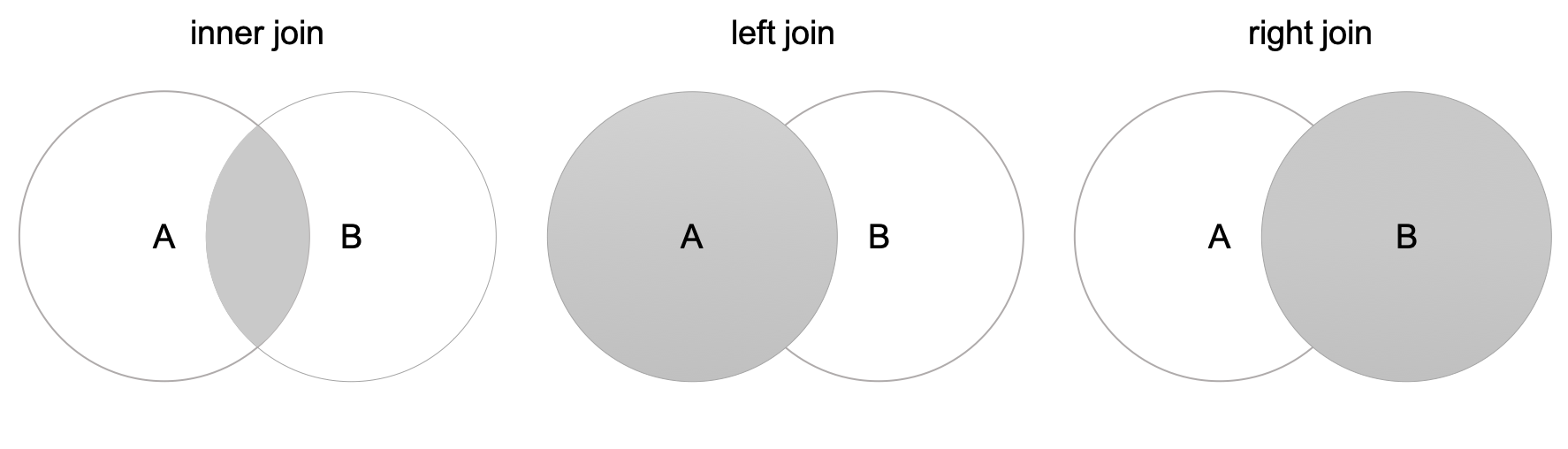
Join6 combines columns from one or more tables for RMDBs. We also have the Join operation available in data.table and pandas. We only talk about 3 different types of joins here, .i.e., inner join, left join, and right join. Left join and right join are also referred as outer join.
Let’s make two tables to join.
 1 > department_dt=data.table(department_id=c(1, 2, 3), department_name=c("Engineering","Operations","Sales"))
 2 > department_dt
 3    department_id department_name
 4 1:             1     Engineering
 5 2:             2      Operations
 6 3:             3           Sales
 7 > employee_dt=data.table(employee_id=c(1,2,3,4,5,6), department_id=c(1,2,2,3,1,4))
 8 > employee_dt
 9    employee_id department_id
10 1:           1             1
11 2:           2             2
12 3:           3             2
13 4:           4             3
14 5:           5             1
15 6: 6 4 1 >>> department_df=pd.DataFrame({'department_id':[1,2,3], 'department_name':["Engineering","Operations","Sales"]})
2 >>> department_df
3 department_id department_name
4 0 1 Engineering
5 1 2 Operations
6 2 3 Sales
7 >>> employee_df=pd.DataFrame({'employee_id':[1,2,3,4,5,6], 'department_id':[1,2,2,3,1,4]})
8 >>> employee_df
9 employee_id department_id
10 0 1 1
11 1 2 2
12 2 3 2
13 3 4 3
14 4 5 1
15 5 6 4We can join tables with or without the help of index/key. In general, joining on index/key is more fast. Thus, I recommend always to set key/index for join operations.
 1 > setkey(employee_dt,'department_id')
 2 > setkey(department_dt,'department_id')
 3 > department_dt[employee_dt] # employee_dt left join department_dt
 4    department_id department_name employee_id
 5 1:             1     Engineering           1
 6 2:             1     Engineering           5
 7 3:             2      Operations           2
 8 4:             2      Operations           3
 9 5:             3           Sales           4
10 6:             4            <NA>           6
11 > department_dt[employee_dt,nomatch=0] # employee_dt left join department_dt
12    department_id department_name employee_id
13 1:             1     Engineering           1
14 2:             1     Engineering           5
15 3:             2      Operations           2
16 4:             2      Operations           3
17 5:             3           Sales           4
18 > employee_dt[department_dt] # employee_dt right join department_dt
19    employee_id department_id department_name
20 1:           1             1     Engineering
21 2:           5             1     Engineering
22 3:           2             2      Operations
23 4:           3             2      Operations
24 5:           4             3           Sales
To join data.table A and B, the syntax A[B] and B[A] only work when the keys of A and B are set. The function merge from data.table package works with or without key.
 1 > # merge function works with keys
 2 > merge(employee_dt,department_dt,all.x=FALSE,all.y=FALSE) # inner join
 3    department_id employee_id department_name
 4 1:             1           1     Engineering
 5 2:             1           5     Engineering
 6 3:             2           2      Operations
 7 4:             2           3      Operations
 8 5:             3           4           Sales
 9 > merge(employee_dt, department_dt, all.x=TRUE, all.y=FALSE) # employee_dt left join department_dt
10    department_id employee_id department_name
11 1:             1           1     Engineering
12 2:             1           5     Engineering
13 3:             2           2      Operations
14 4:             2           3      Operations
15 5:             3           4           Sales
16 6:             4           6            <NA>
17 > merge(employee_dt, department_dt,all.x=FALSE,all.y=TRUE) # employee_dt right join department_dt
18    department_id employee_id department_name
19 1:             1           1     Engineering
20 2:             1           5     Engineering
21 3:             2           2      Operations
22 4:             2           3      Operations
23 5:             3           4           Sales
24 > # merge function works without keys
25 > setkey(employee_dt,NULL)
26 > setkey(department_dt,NULL)
27 > department_dt[employee_dt]
28 Error in `[.data.table`(department_dt, employee_dt) :
29   When i is a data.table (or character vector), the columns to join by must be specified either using 'on=' argument (see ?data.table) or by keying x (i.e. sorted, and, marked as sorted, see ?setkey). Keyed joins might have further speed benefits on very large data due to x being sorted in RAM.
30
31 > merge(employee_dt,department_dt, all.x=FALSE, all.y=FALSE, by.x='department_id',by.y='department_id')
32    department_id employee_id department_name
33 1:             1           1     Engineering
34 2:             1           5     Engineering
35 3:             2           2      Operations
36 4:             2           3      Operations
37 5:             3           4           Sales
The join operations for data.table are summarized in table below.
| type | syntax 1 | syntax 2 |
| A inner join B | A[B, nomatch=0] or B[A, nomatch=0] | merge(A, B, all.x=FALSE, all.y=FALSE) |
| A left join B | B[A] | merge(A, B, all.x=TRUE, all.y=FALSE) |
| B right join A | A[B] | merge(A, B, all.x=FALSE, all.y=TRUE) |
In pandas, there are also different ways to join DataFrame. Let’s just focus on the basic method with the merge function (other methods may also be based on this function).
 1 >>> department_df.set_index('department_id', inplace=True)
 2 >>> employee_df.set_index('department_id', inplace=True)
 3 >>> pd.merge(employee_df, department_df, how='inner', left_index=True, right_index=True) # inner join on index
 4                employee_id department_name
 5 department_id
 6 1                        1     Engineering
 7 1                        5     Engineering
 8 2                        2      Operations
 9 2                        3      Operations
10 3                        4           Sales
11 >>> pd.merge(employee_df, department_df, how='left', left_index=True, right_index=True) # left join on index
12                employee_id department_name
13 department_id
14 1                        1     Engineering
15 1                        5     Engineering
16 2                        2      Operations
17 2                        3      Operations
18 3                        4           Sales
19 4                        6             NaN
20 >>> pd.merge(employee_df, department_df, how='right', left_index=True, right_index=True) # right join on index
21                employee_id department_name
22 department_id
23 1                        1     Engineering
24 1                        5     Engineering
25 2                        2      Operations
26 2                        3      Operations
27 3                        4           Sales
28 >>> employee_df.reset_index()
29 >>> department_df.reset_index()
30 >>> pd.merge(employee_df, department_df, how='inner', left_on='department_id', right_on='department_id') # join with columns directly (not on index)
31                employee_id department_name
32 department_id
33 1                        1     Engineering
34 1                        5     Engineering
35 2                        2      Operations
36 2                        3      Operations
37 3                        4           Sales
We have learned the very basics of data.table and pandas. In fact, there are lots of other useful features in both tools which are not covered in this chapter. For example, the .I/.N symbol in data.table, and the stack/unstack method in pandas.
1 https://arrow.apache.org
2 https://github.com/modin-project/modin
3 https://en.wikipedia.org/wiki/SQL
4 https://en.wikipedia.org/wiki/Comma-separated_values
5 https://www.python.org/dev/peps/pep-0448
6 https://en.wikipedia.org/wiki/Join_(SQL)